系统优化中期作业

文章导航

× 文章目录

1. 1. Project Requirement
2. 2. Problem
3. 3. Main method
4. 4. Results and analysis
5. 5. Program
   1. 5.1. Matlab program
   2. 5.2. Python program

研一上系统优化中期作业，优化求解。

Project Requirement

1. Give a non-quadratic nonlinear objective function and linear inequality constraints (at least two).

2. Select a computational method (primal or dual) for constrained optimization you learn in the class.

3. Show your computational results and corresponding analysis.

4. Submit the typed report.

5. Attach your program

Problem

Consider the problem below:

We solve this problem by using Lagrangian Relaxation Method.

Main method

When we use the Lagrangian Relaxation Method, we describe the problem as below, the i-th equality constrain is expressed as while the i-th inequality constrain is expressed as

So the unconstrained optimization problem can be described as:

We can construct the Joseph-Louis Lagrange operator function, then the necessary conditions for the optimal solution can be obtained.

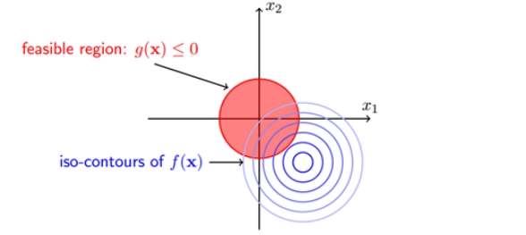
It can be found that when the constrained plane is tangent to the equipotential surface, the gradient orthogonality on the equipotential line and the gradient orthogonality on the constrained plane are both on the same tangent plane, so the two gradients are expressed linearly. In other words, we can express each other with a coefficient, which we usually call the Lagrangian multiplier.

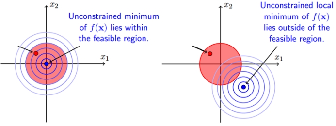
When the constrained area contains the original feasible solution of the objective function, and the feasible solution of the constrained is still inside the constrained area at this time, corresponding to the case of g(x)<0, then the constrained condition does not work; when the constrained area is not When the original feasible solution of the objective function is included, the feasible solution falls on the boundary g(x)=0 after adding constraints. The following figure describes the two cases respectively. The right figure shows that the feasible solution with the constraint will fall on the boundary of the constraint region.

So we know that in either case the expression below always holds:

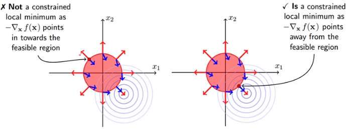
If λ≠0, this means that the feasible solution x falls on the boundary of the constrained region. At this time, the feasible solution should be as close as possible to the unconstrained solution, so on the constrained boundary, the negative gradient direction of the objective function should be far away from the constrained region Towards the unconstrained solution, the gradient direction of the constraint function is exactly the same as the negative gradient direction of the objective function:

This solution also holds in equation constrains, thus we get the KKT conditions:

Our problem has non-quadratic nonlinear objective function and linear inequality constraints. So we can rewrite the unconstrained optimization problem as:

Where equal to the above. The KKT conditions can be rewrite as:

Results and analysis

Step1: Write the Lagrange function:

Step2: Get the partial derivative of :

Step3: Relax constrain2, that means .

We get the equation:

Solve this equation, we get: x1 = 0.157380, x2 = 5.098362,

= -1.316836, = -20.983589,

Constrain2: = -9.963951 < 0

The results meet constraint2 and x1,x2 > 0, but < 0 doesn’t meet KKT condition (4), so they are *not* optimal solutions.

Step4: Relax constrain1, that means .

We get the equation:

Solve this equation, we get: x1 = 0.252336, x2 = 4.346513,

= 1.139798, = -30.866020,

Constrain1: = -6.489574 < 0

The results meet constraint1, x1,x2 > 0 and > 0 meets KKT condition (4), so they are optimal solutions.

Step5: Conclusion

We obtain that when the point is (0.252336, 4.346513), the objective function reaches the minimum value: -30.866020.

Test1

We use function fmincon in Matlab and function minimize in Python to solve the nonlinear programming. The results are written below:

In Matlab, we get the optimal solution is (0.2523, 4.3465), the minimum value is -30.8660.

In Python, we get the optimal solution is (0.252332, 4.346513), the minimum value is -30.866020.

So the results we get is correct!

Test2

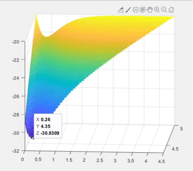
We draw the corresponding 3D picture of the objective function, points witch don’t satisfy the constrains were deleted. The minimum point is very close to (0.26, 4.35), and the minimum value is close to -30.8309.

Program

Matlab program

x = 0:.01:5;y = 0:.01:5;
[x,y] = meshgrid(x,y);
f=-20.*exp(-3*x).*x-18.*exp(0.75*(3-y)).*y;
f(-5*x+8*y-40 > 0 | 2*x-13*y+56 > 0) = nan;
mesh(x,y,f)
clear;
%% 使用matlab自带优化函数求解
function fy = f(x)
  fy =-20*(exp(-3*x(1)))*x(1)-18*(exp(0.75*(3-x(2))))*x(2);
end
[x,y]=fmincon('f',[0 0],[-5 8;2 -13],[40;-56],[],[],[0 0],[])
%% 拉格朗日乘子法求最优化解
% 用syms表示变量构造拉格朗日函数
syms x y lama1 lama2
f1=-20*(exp(-3*x))*x-18*(exp(0.75*(3-y)))*y+lama1*(-5*x+8*y-40);
f2=-20*(exp(-3*x))*x-18*(exp(0.75*(3-y)))*y+lama2*(2*x-13*y+56);
% 分别求f1函数关于 x1、y1、lama1；f2函数关于 x2、y2、lama2的偏导
dx1=diff(f1,x);
dy1=diff(f1,y);
dlama1=diff(f1,lama1);
dx2=diff(f2,x);
dy2=diff(f2,y);
dlama2=diff(f2,lama2);
% 分别令两个约束之一无效（可行解在约束区域内），研究结果
[x1, y1, lama1]=solve(dx1,dy1,dlama1,x,y,lama1)
result1=-20*(exp(-3*x1))*x1-18*(exp(0.75*(3-y1)))*y1
test1 = 2*x1-13*y1+56 % 测试约束2是否满足
[x2, y2, lama2]=solve(dx2,dy2,dlama2,x,y,lama2)
result2=-20*(exp(-3*x2))*x2-18*(exp(0.75*(3-y2)))*y2
test2 = -5*x2+8*y2-40 % 测试约束1是否满足

Python program

from scipy.optimize import minimize
import numpy as np

# 待优化非线性函数：
def func(args):
    fun = lambda x: -20*x[0]*np.exp(-3*x[0])-18*x[1]*np.exp(0.75*(3-x[1]))
    return fun

# 各种约束
def con(args):
    cons = ({'type': 'ineq', 'fun': lambda x: 5*x[0]-8*x[1]+40},
           {'type': 'ineq', 'fun': lambda x: -2*x[0]+13*x[1]-56})
    return cons


if __name__ == "__main__":
    args = ()
    args1 = ()
    cons = con(args1)
    x0 = np.array((2.0, 1.0))  # 设置初始值

    # 调用默认包求解
    res = minimize(func(args), x0, method='SLSQP', constraints=cons)
    print(res.success)
    print("x1=", res.x[0], ";  x2=", res.x[1])
    print("最优解为：", res.fun)